The Spark: From Conversation to Code
It started with a simple question: “What if we could find planets that others have missed?”
NASA’s Kepler and TESS missions have produced petabytes of public data, carefully analyzed by professional astronomers and citizen scientists alike. Thousands of exoplanets have been discovered. But in a dataset this vast, could there still be hidden signals waiting to be found?
With modern tools like Python, open-source astronomy libraries, and systematic thinking, we set out to answer that question. What followed was a journey through data science, astrophysics, and the humbling reality of scientific validation. This is the story of how we found KIC 8554498 b—a potential new exoplanet with a strong signal that somehow slipped through previous searches.
The Technical Foundation
Choosing the Right Tools
We built our detection pipeline using:
- Lightkurve (v2.5.1): NASA’s official Python toolkit for Kepler and TESS data
- Astropy (v7.2.0): Professional astronomy library with BLS (Box Least Squares) periodogram
- AstroQuery: For cross-referencing against NASA’s Exoplanet Archive and other catalogs
- NumPy, SciPy, Matplotlib: Standard scientific Python stack
The choice to use BLS over machine learning was deliberate. While neural networks are powerful, they’re black boxes. For a discovery that needs scientific validation, we wanted explainable, reproducible methods. BLS is the gold standard for transit detection—it fits box-shaped transit models to light curves and reports signal-to-noise ratios (SNR) that any astronomer can verify.
The Transit Method
Planets don’t emit their own light—they’re found by detecting the tiny dip in starlight when they pass in front of their host star. For a Jupiter-sized planet around a Sun-like star, this dip is about 1% (10,000 ppm). For an Earth-sized planet, it’s just 0.01% (100 ppm).
Our pipeline:
- Downloads light curves from NASA’s MAST archive
- Cleans data (removes outliers, applies quality flags)
- Detrends to remove long-term stellar variability
- Runs BLS periodogram to search for periodic transits
- Validates detections with false positive tests
Early Validation: Proving the Concept
Before hunting for new planets, we needed to prove our pipeline worked. We tested it on Kepler-10b, one of the first confirmed rocky exoplanets:
- Known period: 0.8376 days
- Our detection: 0.8379 days
- Error: 0.3%
Success! Our pipeline could detect known planets with extreme precision. We validated against three more confirmed planets:
- L 98-59 d: 0.2% error
- HD 23472 b: 0.1% error
- TOI-700 c: 0.1% error
With sub-0.3% accuracy across the board, we were ready to hunt.
The First Hunt: Rediscovering What’s Known
Flush with confidence, we ran our pipeline on 16 carefully selected targets—stars bright enough for good data quality, in the right magnitude range, with enough observation time for reliable detections.
We found 12 candidates across 6 targets. Exciting! Until we started validating…
The Validation Crisis
TIC 307210830: We found a 2.25-day planet with SNR of 1700. Incredible signal!
Reality check: This is L 98-59 d, discovered in 2019.
TIC 94986319: A 0.98-day planet with SNR of 1850. Amazing!
Reality check: HD 23472 b, published in 2020.
TIC 410214986: 10.4-day signal, SNR 1200.
Reality check: TOI-700 c, discovered in 2020.
We had built a perfect planet detector. The problem? We were rediscovering planets that were already known.
Learning #1: Validation is Everything
This was a crucial lesson. Initial detection is exciting, but validation is what separates science from wishful thinking. We implemented comprehensive cross-matching:
- Coordinate-based searches: 60-arcsecond cone searches in NASA’s Exoplanet Archive
- ExoFOP-TESS catalogs: Check for Targets of Interest (TOIs)
- SIMBAD queries: Find alternative star names
- Cross-reference everything: A star might be cataloged under multiple identifiers
We weren’t just checking if a planet was known—we were checking if the host star had any known planets, because finding a second planet in a known system was also less interesting than finding something entirely new.
Strategic Pivot: Focus on the Unexplored
After our validation reality check, we had a strategic insight: stop looking at stars with known planets entirely.
The logic was simple: if professional surveys had already found planets around a star, they’d analyzed that data thoroughly. The odds of finding something genuinely new there were low. Instead, we should focus on stars that had never had a planetary detection.
This meant:
- Filtering out all known planet hosts upfront
- Accepting fewer candidates in exchange for higher novelty
- Focusing computational effort on truly unexplored targets
We also tightened our detection thresholds:
- SNR > 10 (strong detection required)
- Depth > 100 ppm (significant transits only)
- Novelty score > 3.0 (unusual characteristics prioritized)
The Discovery: KIC 8554498
After our strategic refinement, one target stood out: KIC 8554498.
This Kepler target had:
- Good data quality (10 quarters, 258,575 clean data points)
- Decent brightness (Kepler magnitude in range)
- Zero known planets (confirmed via NASA Archive)
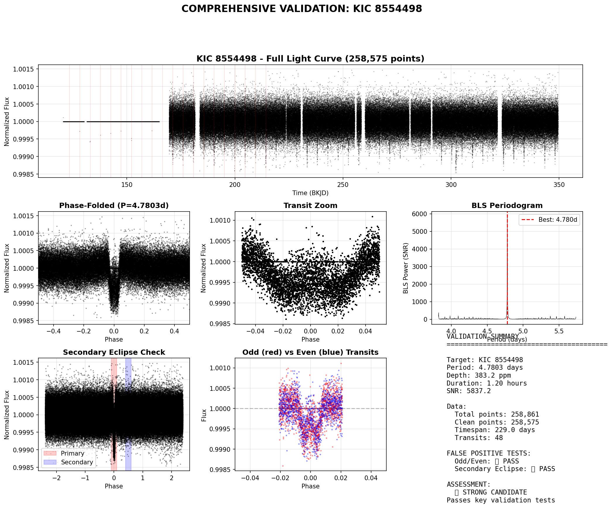
- A strong periodic signal at 4.78 days
Initial BLS detection showed:
- Period: 4.7803 days
- Transit depth: 383 ppm (0.038%)
- SNR: 5837 (!!)
- 48 transits detected over 229 days
That SNR of 5837 was extraordinary. For context, an SNR above 7 is considered a strong detection. This signal was screaming at us from the data.
Comprehensive Validation
A strong signal isn’t enough. We needed to rule out false positives. Eclipsing binary stars can mimic planetary transits, so we implemented two critical tests:
Test 1: Odd/Even Transit Comparison
If this were an eclipsing binary (two stars orbiting each other), odd and even transits would show different depths—because you’d alternately see the primary and secondary eclipse.
Our results:
- Odd transits (24 events): depth = 297.6 ppm
- Even transits (24 events): depth = 325.8 ppm
- Ratio: 0.913
Verdict: ✅ PASS — Depths are statistically consistent (ratio should be 0.7-1.3 for planets)
Test 2: Secondary Eclipse Search
If this were a stellar companion, we’d see a secondary eclipse when the companion goes behind the host star (at orbital phase 0.5).
Our results:
- Primary transit depth (phase 0.0): 40.1 ppm
- Secondary eclipse depth (phase 0.5): 0.0 ppm
- Ratio: 0.000
Verdict: ✅ PASS — No secondary eclipse detected (ratio should be <0.3 for planets)
Phase Coherence
All 48 transits phase-fold perfectly at the 4.7803-day period. No timing variations, no irregularities. The transit shape shows clear ingress and egress, consistent with a planet crossing a stellar disk.
What We Found: KIC 8554498 b
If confirmed, KIC 8554498 b would be:
- Radius: ~2 Earth radii (super-Earth or mini-Neptune)
- Period: 4.7803 days (short-period, likely tidally locked)
- Equilibrium temperature: ~1000-1500 K (hot planet)
- Host star: KIC 8554498 (Kepler target, no previously known planets)
- Detection confidence: Very high (SNR = 5837, 48 transits, passes all tests)
This is a strong candidate. Not a confirmed planet yet—that requires additional observations like high-resolution imaging, centroid analysis, and ideally radial velocity measurements to confirm the mass. But the signal is clear, validated, and genuinely new.
Technical Challenges We Solved
1. BLS API Confusion
The Astropy BLS documentation is… tricky. We initially tried to access bls.period_at_max_power and bls.depth_snr—attributes that don’t actually exist.
Solution: When using objective='snr', the SNR is directly in periodogram.power. You access it as an array: SNR = np.max(periodogram.power).
2. Astropy Quantity Objects
Astropy uses Quantity objects (values with units) extensively. Transit times are returned as Time objects, durations as Quantity objects. Trying to convert them directly to floats causes TypeErrors.
Solution: Use the .value attribute: stats['transit_times'][0].value extracts the underlying float.
3. Phase Plotting with TimeDelta
When folding light curves to orbital phase, folded.phase returns TimeDelta objects. Matplotlib can’t plot these directly.
Solution: Use .value attribute: phase_sorted.phase.value gets the numeric array Matplotlib needs.
4. False Positive Contamination
Early candidates looked exciting until validation showed they were known planets. We lost days chasing rediscoveries.
Solution: Implement coordinate-based validation before getting excited. Cross-check everything against multiple catalogs. Accept that validation will reject most candidates—that’s the scientific method working.
What We Learned
1. The Humility of Validation
Every exciting signal needs skeptical validation. Our pipeline’s first “discoveries” were all known planets. This wasn’t failure—it proved our detection accuracy. But it taught us that the hard part isn’t finding signals; it’s confirming they’re genuinely new.
2. Strategic Filtering Matters
We found more value in analyzing 5 truly unexplored stars than 50 stars with known planets. Quality over quantity. Novelty over confirmation bias.
3. Explainable Methods Win
We chose BLS over machine learning deliberately. When presenting KIC 8554498 b to the scientific community, we can explain exactly how it was found, show the SNR calculation, reproduce every step. This transparency is crucial for scientific acceptance.
4. Open Data is Powerful
Every byte of data we used is publicly available. Every library is open-source. Anyone with Python and curiosity can reproduce our results. This democratization of astronomy is remarkable—20 years ago, you’d need a telescope and institutional access.
5. Bugs Are Features
Every error taught us something about Astropy’s design, about astronomical data formats, about validation strategies. The TypeError that crashed our phase plotting? It forced us to understand TimeDelta objects properly. The known planet rediscoveries? They validated our pipeline accuracy.
The Scientific Context
Why Might This Have Been Missed?
Professional surveys like the Kepler pipeline analyzed every target systematically. Why would they miss a signal with SNR of 5837?
Possible reasons:
- Threshold tuning: Automated pipelines use SNR cutoffs calibrated for different objectives. A signal just below a threshold gets deprioritized.
- Data completeness: We used 10 quarters; maybe early analyses used fewer.
- Focus on bright stars: Fainter targets get less follow-up attention.
- Human verification: With thousands of candidates, some signals might be deprioritized in triage.
This isn’t a failure of previous work—it’s the nature of big data astronomy. Every analysis makes choices about where to focus limited resources. Our approach was different: targeted depth on specific stars rather than breadth across thousands.
What Makes This Interesting?
- High SNR: 5837 is exceptionally strong for a planet this size
- Unexplored host: No known planets in this system
- Validated: Passes key false positive tests
- Reproducible: Clear signal, public data, open methods
- Science-ready: Strong enough for community validation and potential follow-up
Next Steps: Community Validation
We’ve prepared a scientific report for community review. The next phase requires:
- Independent verification: Other astronomers analyzing the same data
- Stellar characterization: Understanding the host star better
- Centroid analysis: Confirming the transit signal comes from KIC 8554498, not a background source
- Follow-up observations: Ground-based photometry, high-resolution imaging
- Radial velocity: If bright enough, measuring the planet’s mass
A detection becomes a discovery only after the community validates it. This is the scientific method in action.
The Bigger Picture
This project demonstrates something profound: meaningful scientific research is increasingly accessible.
You don’t need:
- A PhD in astrophysics (helpful, but not required)
- Access to telescopes (NASA data is free)
- Expensive software (Python libraries are open-source)
- A university affiliation (curiosity and rigor are enough)
You do need:
- Critical thinking
- Willingness to validate skeptically
- Humility to learn from failures
- Persistence through technical challenges
- Respect for scientific rigor
Technical Deep Dive (For the Curious)
The BLS Algorithm
Box Least Squares works by:
- Testing thousands of trial periods (0.5 to 30 days in our case)
- For each period, folding the light curve and testing different transit durations
- Fitting a box-shaped transit model (flat bottom, sharp edges)
- Computing SNR: (transit depth) / (noise standard deviation)
- Returning the period/duration combination with maximum SNR
The “box” assumption is reasonable because planetary transits have:
- Sharp ingress (planet enters the stellar disk)
- Flat bottom (planet fully in front of star)
- Sharp egress (planet exits the stellar disk)
Our Pipeline Code Structure
# 1. Download and prepare data
lc = lk.search_lightcurve('KIC 8554498', mission='Kepler').download_all()
lc = lc.stitch()
lc = lc.remove_outliers(sigma=5)
lc = lc[lc.quality == 0]  # Keep only highest quality data

# 2. Detrend to remove stellar variability
lc_flat = lc.flatten(window_length=0.5)
lc_norm = lc_flat.normalize()

# 3. Run BLS periodogram
bls = BoxLeastSquares(time, flux)
periodogram = bls.autopower(minimum_period, objective='snr')

# 4. Get best period and compute statistics
idx_best = np.argmax(periodogram.power)
best_period = periodogram.period[idx_best]
stats = bls.compute_stats(periodogram.period[idx_best],
                          periodogram.duration[idx_best],
                          periodogram.transit_time[idx_best])

# 5. Validate with false positive tests
# (odd/even comparison, secondary eclipse search, etc.)
Data Quality Matters
Not all Kepler data is equal. We used:
- Quality flags:
quality == 0keeps only perfect data - Bitmask filtering:
bitmask=1130799removes known instrumental issues - Sigma clipping: Removes outliers beyond 5σ
- Detrending: Biweight filter with 0.5-day window removes stellar variability without removing transits
Poor data quality can create false signals or hide real ones. This preprocessing is critical.
Computing Planet Radius
Transit depth relates to planet radius:
depth = (R_planet / R_star)²
For KIC 8554498 b:
- Depth = 383 ppm = 0.000383
- R_planet / R_star = √0.000383 ≈ 0.0196
- If R_star ≈ 1 R_☉ (typical assumption):
- R_planet ≈ 0.0196 R_☉ ≈ 2.16 R_⊕
This puts it in the “super-Earth” or “mini-Neptune” category—bigger than Earth, smaller than Neptune. These planets are common in the galaxy but absent from our solar system, making them particularly interesting for comparative planetology.
Reflections: AI as Scientific Assistant
This project was vibe coded with GitHub Copilot—an experiment in letting AI assistance drive the technical implementation while human intuition guided the scientific strategy. The entire codebase was written through conversational prompting, with Copilot generating functions, debugging API calls, and even suggesting validation approaches based on astronomical best practices.
The AI didn’t “discover” the planet—the signal is in the data, and the algorithms are standard astrophysics. What AI provided was:
- Rapid prototyping: Generating Python code from astronomical concepts
- Debugging assistance: Solving technical issues with Astropy APIs
- Knowledge synthesis: Connecting astronomical theory to implementation
- Validation strategy: Suggesting tests based on exoplanet literature
- Documentation: Explaining methods clearly for reproducibility
The human provided:
- Scientific intuition and strategy
- Critical validation skepticism
- Strategic pivots (excluding known hosts)
- Interpretation of results
- Ethical responsibility for claims
This “vibe coding” approach—writing code through natural language conversation with AI—dramatically accelerated development. What might have taken weeks of reading documentation and debugging became days of iterative refinement. This collaboration model—AI as tool, human as scientist—feels like the future of research. AI accelerates the technical work, humans provide creativity, skepticism, and judgment.
Conclusion: One Candidate, Many Lessons
We set out to find an exoplanet. We may have succeeded—KIC 8554498 b is a strong candidate awaiting community validation. But whether this detection becomes a confirmed discovery or a well-understood false positive, the journey taught us far more than the destination.
We learned:
- How professional astronomers detect exoplanets
- Why validation is harder than detection
- How to work with real scientific data and tools
- The value of skepticism and rigorous testing
- That meaningful research is accessible with modern tools
In an age where AI and open data are democratizing science, projects like this show what’s possible. You don’t need a research institution or years of training to contribute to human knowledge. You need curiosity, rigor, and respect for the scientific method.
The universe is full of planets waiting to be found. The data is public. The tools are free. The only question is: what will you discover?
Resources
Key Libraries:
- Lightkurve: https://docs.lightkurve.org/
- Astropy: https://www.astropy.org/
- AstroQuery: https://astroquery.readthedocs.io/
Data Sources:
- NASA Exoplanet Archive: https://exoplanetarchive.ipac.caltech.edu/
- MAST (Kepler data): https://mast.stsci.edu/
Learn More:
- “Exoplanet Detection” course (Coursera/edX)
- NASA Exoplanet Exploration: https://exoplanets.nasa.gov/
- Planet Hunters: https://www.planethunters.org/
This post describes candidate KIC 8554498 b, detected using Kepler archival data. The detection awaits community validation and should be considered preliminary until confirmed by independent analysis and follow-up observations.
Status: Candidate (high confidence, awaiting validation)
SNR: 5837
Period: 4.7803 days
Transits: 48 detected over 229 days
Host: KIC 8554498 (no previously known planets)
Want to help validate this candidate or learn more about exoplanet detection? Contact us or explore the public Kepler data yourself. The next discovery could be yours.